10 Tips To Souping Up Rmarkdown

Souping up R Markdown!

For folks that are just getting started in R, or for those who have so far avoided doing anything that isn’t just coding in R, I wanted to jot down a few tips that I’ve found useful when working with the magic that is Rmarkdown!

This is not meant to be a comprehensive tutorial, and it may not even be useful to you, but it may highlight a few new things you can try, or inspire you to at least jump into the world of Rmarkdown. It’s really transformed the way I do analysis, communicate, create websites, write, etc. For actual details on souping up RMarkdown, see http://rmarkdown.rstudio.com, or any of the other great resources that actual experts have written.

But for now let’s soup it up!

10 Tips to Soup things Up

Here’s an internally linked list to the sections! To link, you can add a {#custom_label_here} at the end of the section title. Something like ## My Section {#custom_label_here} and then reference as [a section name](#custom_label_here).

Using knitr::include_graphics for all figures

Using the here::here() package & changing figure sizes

Adding logos/images in your title or header/footer

Show the R code chunks verbatim

Including variables in R chunks from other R chunks!

Icons and Emojis

Interactive Plots

Sourcing other scripts to generate content

Making columns in Rmarkdown

Maps Maps Maps!

1. Using `knitr::include_graphics` and `here::here()`

This one is something I use pretty much always. It has made things soo much easier in many ways. It’s also very flexible. By calling a graphic (could be a figure, picture, plot, whatever) inside an R-chunk with knitr::include_graphics() instead of using the markdown syntax (![](path/to/figure)), you can control the size, placement, etc etc. Even better, when you are using RStudio projects, you can use relative pathnames to a file on your computer instead of having to deal with the pain of using the .. to signify going “up” a directory outside of the place the .Rmd lives. Zev Ross has a great post showing how to resize and customize images and figures in Rmarkdown…check it out here.

For example, let’s look at this picture of a can of soup, using a weblink.

From a url

# straight from web:
knitr::include_graphics('https://upload.wikimedia.org/wikipedia/commons/thumb/5/5f/Can%2C_food_%28AM_2007.41.2-1%29.jpg/766px-Can%2C_food_%28AM_2007.41.2-1%29.jpg')

a beatiful can of soup from a web URL

2. Using `here::here()`

We’re going to do the same thing as above, but we’ll use a path to a file on my computer. The trick here is Rmd has the helpful ^(?) habit of defaulting to the directory it lives in…so anything not in the same folder as your .Rmd file requires some extra redirection before you click Knit. Otherwise the computer can’t find whatever it is you want plotted/printed.

Enter the great package {here}. Please go look just to see Allison Horst’s awesome art. Anyway, we can use the here::here() syntax to keep the path relative and avoid things breaking, or having to change all the setwd() type links.

Here we can also tweak the size of our photo and placement inside the header of the R chunk. Here’ I’m adding these options to my code chunk:


```{r knitrsoupTst, fig.cap= "a beatiful can of soup from a local file", echo=TRUE, eval=TRUE, out.width='25%', fig.align='left'}
```

Note, the out.width='25%' and fig.align='left' options here. They allow us to change the size of our figure as well as the location.

# download.file(url="https://upload.wikimedia.org/wikipedia/commons/thumb/5/5f/Can%2C_food_%28AM_2007.41.2-1%29.jpg/766px-Can%2C_food_%28AM_2007.41.2-1%29.jpg", destfile = "img/toheroa_soup.jpg")

# now wrap with paste0()
knitr::include_graphics(paste0(here::here(), "/img/toheroa_soup.jpg"))

a beatiful can of soup from a local file

3. Add a Logo in your title/header/footer

This is just one demonstration, but there are two parts to this. First, you can include icons in your header or footer! Depending on whether you are outputting an html or pdf file this approach may change slightly, but the basics are here.

For PDF You can include the icon/emblem whatever in your .yaml header. This may look like this:


title: |
  ![](https://upload.wikimedia.org/wikipedia/commons/thumb/5/5f/Can%2C_food_%28AM_2007.41.2-1%29.jpg/766px-Can%2C_food_%28AM_2007.41.2-1%29.jpg){width=0.25in}   
  Souping up R Markdown!
date: "2020-02-20"
output: 
  html_document:
    code_folding: hide

Important : To keep your icon and title on different lines, you’ll want to add 2 spaces at the end of the line with the photo/image. See here for more details: https://bookdown.org/yihui/rmarkdown-cookbook/latex-logo.html

For HTML

This is a bit different. Here we can add a logo by including an R chunk with a path to the logo. We can then specify we want it to live at the top in the header using style = 'position:absolute; top:0; right:0; padding:10px; width:100px. Play with the size with the width: option. For a footer, we can do a similar option but change to: style = 'position:absolute; top:0; right:0; padding:10px; width:100px

htmltools::img(src = knitr::image_uri(file.path(paste0(here::here(), "/img/toheroa_soup.jpg"))), 
               alt = 'logo', 
               style = 'position:absolute; top:0; right:0; padding:10px; width:100px')

For an HTML Footer

For a footer, there’s a great reference here. We’ll need to deal with some html code separately and save it as footer.html. We can then load that into the header of our yaml using something like this:

---
title: "Your title"
output: 
  html_document:
    includes:
      after_body: footer_example.html
---

4. Show R code chunks verbatim

This one is always tricky…the method I’ve found that works (and there are certainly other likely better ways) is to add a small bit to the code chunk. There are two parts, and the link here best describes this. Essentially we need to wrap our whole chunk in 4 backticks on either end. We also need to add a short blank inline R chunk immediately at the end of our R chunk (backtick + r + '' + backtick).

```{r fakecode, eval=FALSE, echo=TRUE}
somecode <- doing_code
```

5. Including variables in R chunks from other R chunks!

This is pretty cool. I saw this tip recently on twitter by Andrew Heiss here, (and thanks Yihui!). We can use variables in code chunks to inform things in other code chunks. For example, let’s play around with the figure size a bit. Maybe instead of specifying figures that we want to be wide will be 7 inches and normal figures will be 75%, we can set those variables at the beginning in a chunk.

# figure sizes
fancy_width <- 7.5
norm75 <- '75%'

Now we can use these in any R chunks following. For example here’s a figure using the norm75 option which is 75% width:


```{r out.width=norm75, fig.cap="75% width"}

mtcars %>% ggplot(.) + geom_point(aes(x=drat, y=wt, color=mpg), size=4) + scale_color_viridis_c()

```

mtcars %>% ggplot(.) + geom_point(aes(x=drat, y=wt, color=mpg), size=4) + scale_color_viridis_c()

75% width

And here’s the fancy_width option:


```{r fig.width=fancy_width, fig.cap="Fancy width"}

mtcars %>% ggplot(.) + geom_point(aes(x=drat, y=wt, color=mpg), size=4) + scale_color_viridis_c()

```

mtcars %>% ggplot(.) + geom_point(aes(x=drat, y=wt, color=mpg), size=4) + scale_color_viridis_c()

Fancy width

6. Emoji & Plots

This isn’t necessarily specific to Rmarkdown, but it’s fun to include emoji’s inside of plots or within the text of an .Rmd.

There are a number of packages now that provide options for using emoji or icons inside of R.

Here we can use something like this:

r icon::fa_r_project(color = "blue")

To give a lovely icon.

Icons in Plots !

Even better, we can use these little bits of flavor in our plots. Since we are really working hard on the soup theme, here’s some fun code that:

scrapes a table from Wikipedia on a list of soups and which country they originated from
Uses the {rvest} package and some {dplyr} to clean up the country names
Counts how many types of soup exist per country (according to this wikipedia table)
Makes a {ggplot} with little soup bowls

## SOUPS

library(rvest)
library(tidyverse)

# wikipedia url about soup types
pg <- read_html("https://en.wikipedia.org/wiki/List_of_soups")

# read in url and get table xpath (highlighted with Inspector in Chrome)
sp_df <- html_nodes(pg, xpath ='//*[@id="mw-content-text"]/div/table') %>% 
  html_table() %>% flatten_df() %>% # go from list to df
  janitor::clean_names() %>% # clean names
  select(-image) %>% 
  dplyr::filter(origin!="") %>% # get rid of blanks
  # clean up names and simplify
  mutate(origin_simple = case_when(
    grepl(x = origin, "Germany") ~ "Germany",
    grepl(x = origin, "India") ~ "India",
    grepl(x = origin,"Indonesia") ~ "Indonesia",
    grepl(x = origin, "Italy") ~ "Italy",
    grepl(x = origin, "^PolandSlovakiaRussiaUkraineCzech") ~ "Eastern Europe",
    grepl(x = origin, "^RussiaUkraine$") ~ "Russia",
    grepl(x = origin, "Greece") ~ "Greece",
    grepl(x = origin, "Spain") ~ "Spain",
    grepl(x = origin, "^UkraineRussia$") ~ "Ukraine",
    grepl(x = origin, "United States|USA") ~ "United States",
    TRUE ~ origin)
  ) %>% 
  # now count how many soups by country
  group_by(origin_simple) %>% add_count() %>% 
  dplyr::filter(n>1)

# PLOT Countries with more than one soup
ggplot() +
  ggimage::geom_image(data=sp_df, aes(x=reorder(origin_simple, n), y=n), image='https://emojipedia-us.s3.dualstack.us-west-1.amazonaws.com/thumbs/240/google/223/bowl-with-spoon_1f963.png') + 
  theme_minimal(base_family = "Roboto Condensed") +
  coord_flip() + 
  scale_y_continuous(breaks = c(seq(0,14,2)))+
  labs(title="Countries with More than One Kind of Soup", 
       subtitle="(According to Wikipedia)",
       caption="* greatly simplified", x="", y="Number of Soup Types")

7. Interactivity in Plotting

When knitting as .html, we have the ability to add some cool interactivity to our plots pretty easily. By using the {plotly} package, and the ggplotly function, we can instantly add the ability to interact with a plot inside the .html file. Let’s make the plot from the last chunk “interactive”. Unfortunately it won’t work with our fun soup bowls, but we can use points instead.

library(plotly)

ggplotly(
  ggplot() +
    geom_point(data=sp_df, aes(x=reorder(origin_simple, n), y=n)) + 
    theme_minimal(base_family = "Roboto Condensed") +
    coord_flip() + 
    scale_y_continuous(breaks = c(seq(0,14,2)))+
    labs(title="Countries with More than One Kind of Soup", 
         subtitle="(According to Wikipedia)",
         caption="* greatly simplified", x="", y="Number of Soup Types")
)

8. Sourcing R scripts Directly into Rmd files

This isn’t something I’ve done much of, but it’s a really interesting way to spin your scripts straight into an Rmarkdown. A great function to play with is the knitr::spin() function. This allows us to directly knit an R script into an Rmd. Check out these resources if you’re interested:

9. Making Columns In an Rmarkdown

Here we can switch from using one giant column across the page, to splitting things into 2 or 3 columns. This can really help make things visually pleasing and allow for side by side plots or text. A basic page is 12 units wide, so you can divide a given page as needed.

Here’s an example. Let’s create a row, which we can fill with whatever, and then split our row into 3 columns.

All about soups

Let’s talk more about soup. One of my favorite soups is a butternut squash soup. Very wholesome, great for winter lunch, or a great first course at family dinners and get-togethers with friends. In particular, using coconut milk as a base with some red thai curry can really make things delicious.

Here’s a delicious picture of some soup

# annual flow on Nile River
Nile %>% as.data.frame() %>% mutate(year=1871:1970) %>% 
  rename(flow=x) %>% 
  ggplot(.)+ geom_line(aes(x=year, y=flow), 
                       color="darkblue", lwd=2) +
  theme_minimal() + labs(x="", y="Flow", 
                         title="Annual river flow on Nile River",
                         subtitle="(1871-1970)")

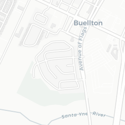
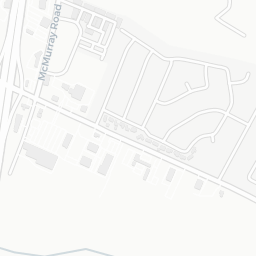
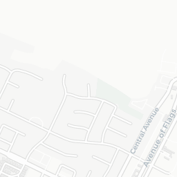
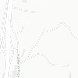
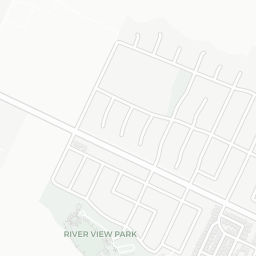
10. Maps Maps Maps

This is sort of cheating because we already had some interactivity in Tip #7. However, we haven’t made any maps, and this is something I commonly share via Rmarkdown because it’s a great way to allow folks to really interact with data they may be interested in playing with.

In particular, the {mapview} and {sf} packages makes this amazingly straight-forward. To make a map that is interactive and fully embedded in a webpage, we can load some or create some data, and then plot it. Here is the split-pea soup capital of the US (according to the google search I just ran).

I’m adding one additional handy bit here which allows you to measure a distance from one thing to any other thing, or draw a polygon and get the area. How far do you live from Buellton? Use the map and find out!

library(mapview)
library(sf)

# create a point to focus on:
# the split-pea soup capital of the US is Buellton California.
buellton <- st_sfc(st_point(c(-120.1927, 34.6136)), crs=4326)

m1 <- mapview(buellton, col.regions="orange") # make the map

# add measure option  
m1@map %>% leaflet::addMeasure(primaryLengthUnit = "meters")